Two workers are quadratically better than one
For latency, anyway.
A common architecture pattern is the “task queue”: tasks enter an ordered queue, workers pop tasks and process them. This pattern is used everywhere from distributed systems to thread pools. It applies just as well to human systems, like waiting in line at a supermarket or a bank. Task queues are popular because they are simple, easy to understand, and scale well.
There are two primary performance metrics for a task queue. Throughput is how many tasks are processed per time unit. Latency is how long a task waits in the queue before being processed. Throughput scales as you’d expect (2x workers ≈ 2x throughput) but latency is less intuitive. For all their popularity, we don’t abstractly model the properties of task queues. We have tools to implement them and tools to trace/metric them, but we don’t use theoretical models to understand our systems in abstract. In this essay we will model a simple task queue and show how the latency is highly sensitive to our initial parameters.
We will be using PRISM to model this problem. PRISM is a probabilistic model checker, meaning it can take a software design and figure out how likely various outcomes are. I’ve talked about PRISM before and criticized it for its restrictive syntax. But here it is the right tool for the job and with some cleverness we can make it shine. This essay will assume no prior knowledge of PRISM. Let’s get started.
Planning Ahead
PRISM supports many different kinds of probabilistic models. The simplest of these is the Discrete Time Markov Process, or dtmc. In this, time progresses one discrete step at the time and everything happens with known probabilities. You can think of it as randomly moving between states of a state machine, where one step is one transition. The step is an abstract amount of time. While you could design under the assumption that each step is a fixed time, like 5 seconds, we don’t need to here.
We will assume that there are N tasks and that they are independent. This means that how long a task takes to process is independent of how many tasks came before and how many tasks come after. However, different tasks will take a different amount of time to process. We can emulate this by flipping it around and saying that each worker has only a certain chance of completing a task each time step. If we say the chance is 50%, then half the tasks will be completed in exactly one step, a quarter will be completed in exactly two, etc. In aggregate, the worker will complete a task roughly every two steps.
PRISM is not expressive enough to let us individually track each task. Fortunately, all the tasks we have are interchangeable: while some tasks will take longer than others to process, this is abstracted away in the probability. We can instead say that there is some integer that represents the number of tasks left, where the worker has a chance each step of decrementing that number. Then if it takes four steps to decrement left, we just say the worker was working on a complex task.
Specifying Throughput
Spec
First some boilerplate:
dtmc //type of model

const int N; // Number of tasks

module workers
  // number of tasks left to process
  // A number between 0 and N
  left : [0..N] init N;
We need to make a command to represent the worker completing a task. First the full command, then the breakdown of how it works:
  [worker] (left > 0) ->
        0.5: (left' = left - 1)
        + 0.5: true;
Commands have three parts: a label, a guard, and an update. We’ll start with the update. We can say this just means that we decrement left. In PRISM syntax, we say that the new value of left, written left', is left - 1
(left' = left - 1)
But it only succeeds 50% of the time. The other 50% of the time nothing happens. We could write queue' = queue, or we can use the shorthand true:
0.5: (left' = left - 1) + 0.5: true;
Next is the guard. The update is only possible if the guard is true. The obvious guard we need here is that we can’t work on a task if there aren’t any tasks left. That leaves just the label, which is an optional name we give to the command.
It’s good form to leave a “stutter state” at the end so that the model doesn’t deadlock. So if we’re out of tasks, we just say true.
  [worker] (left > 0) ->
        0.5: (left' = left - 1)
        + 0.5: true;

 [] (left = 0) -> true;
endmodule
Full spec:
show spec
dtmc

const int N; // Number of tasks

module workers
  left : [0..N] init N;

  [worker] (left > 0) ->
        0.5: (left' = left - 1)
        + 0.5: true;
  [] (left = 0) -> true;

endmodule

// see next section
rewards "total_time"
  [] left > 0: 1;
endrewards
Modeling Throughput
In programs, we have one level of coding: the program itself. With specifications, we have two levels. We write the specs and then we write the properties about the specs. In PRISM we can also write properties as queries on the system and have the model checker tell us what the expect values are.
Our first property is the total time taken to process all tasks. To track this we need to make a small change to our spec. A reward function is a value we assign to each successive state in the evolution of the system. This will become much more important when we need to model latency, but for now we can get away with a very simple reward function:
rewards "total_time"
  [] left > 0: 1;
endrewards
If there are any tasks left in the queue, we increment the total reward for that behavior by one.1 The total reward is the number of steps taken to complete all tasks.
Next we need a property that gets us the reward at the moment we run out of tasks. That looks like this:
// reward in first state where left = 0
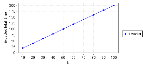
R{"total_time"}=? [ F left=0 ]
The reward will depend on the number of tasks we start with, or N. We can run an experiment, where we test the property for a set of N and graph the result. Here’s the throughput for N from 10 to 100, in steps of 10:
show data
| N | Result |
|---|---|
| 10 | 20 |
| 20 | 40 |
| 30 | 60 |
| 40 | 80 |
| 50 | 100 |
| 60 | 120 |
| 70 | 140 |
| 80 | 160 |
| 90 | 180 |
| 100 | 200 |
That gives us throughput. But our model can’t tell us anything about latency yet, because we’ve assumed that all of the tasks start out in the queue. That models a batch process, not tasks coming in over time and waiting till their turn.
This is where latency becomes very important. In addition to how long it takes to process a task, we want to account for how long tasks are waiting before being processed. Our model is incomplete until we add this in.
Specifying Latency
Spec
Instead of all the tasks being available for work immediately, we say that they come in over time. We add a new variable, queue, to represent the number of tasks actually present in the queue. We also add an enqueue command that adds tasks to the queue if there any left not yet in it. We’ll assume that this happens at the same “rate” the worker processes tasks.This assumption pins us to a specific subset of the configuration space.2 It’s fine for now, but we’ll eventually want a more general specification.
  queue: [0..N] init 0;
  [enqueue] (queue < left) ->
    0.5: (queue' = queue + 1)
    + 0.5: true;
The worker will only be able to process tasks if the queue is nonempty. When it processes a task, it will decrement from both the total left and the queue.
  [worker] (left > 0 & queue > 0) ->
        0.5: (left' = left - 1) & (queue' = queue - 1)
        + 0.5: true;
Our two commands aren’t exclusive: when 0 < queue < left then both [enqueue] and [worker] are valid commands. In this case, all the possibilities are weighted together. Here this means that there are four equally-likely possibilities:
queueincrementsworkerdecrementsqueuedoes nothingworkerdoes nothing
(3) and (4) have the same outcome, but are different for modeling purposes. In my mental model, worker commands model a longer span of time than enqueue commands do. The worker needs time to process the task, while adding a task to the queue is instantaneous. Since we’re calculating total time taken, we only want to count the worker commands as time passing. We can do this by adding a label to the reward function:
rewards "total_time"
- [] left > 0: 1;
+ [worker] left > 0: 1;
endrewards
Final spec:
show spec
dtmc

const int N; // Number of tasks

module workers
  left : [0..N] init N;
  queue: [0..N] init 0;

  [enqueue] (queue < left) ->
    0.5: (queue' = queue + 1)
    + 0.5: true;

  [worker] (left > 0 & queue > 0) ->
        0.5: (left' = left - 1) & (queue' = queue - 1)
        + 0.5: true;

  [] (left = 0) -> true;


endmodule

// see next section
rewards "wait_time"
  [worker] queue > 1: queue - 1;
endrewards

rewards "total_time"
  [worker] left > 0: 1;
endrewards
Modeling Latency
First, let’s sanity check that we didn’t change the throughput. Since we’re only modeling time passing with worker commands, our new model shouldn’t change the total time. Here’s what we get:
Exactly the same, good. But we’re here to model latency, too. Latency is how long a task waits in the queue before it gets processed. Since we don’t have a way of singling out individual tasks, we can instead look at how long all of the tasks wait in total, which is a correlated value.
The reward function will be similar to total_time, except instead of incrementing the reward by 1, we increment it by queue - 1. We subtract one because if the queue is nonempty then one of the tasks in the queue is being processed.
rewards "wait_time"
  [worker] queue > 0: queue - 1;
endrewards
We also need a new property:
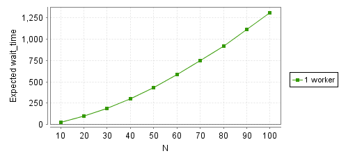
R{"wait_time"}=? [ F left=0 ]
And here’s the latency as a function of N:
show data
| N | Result |
|---|---|
| 10 | 29 |
| 20 | 97 |
| 30 | 190 |
| 40 | 305 |
| 50 | 436 |
| 60 | 584 |
| 70 | 746 |
| 80 | 922 |
| 90 | 1110 |
| 100 | 1310 |
The growth is quadratic! If we have 10 tasks, they wait a total of 30 steps. If we have 100, they wait a total of over 1300 steps. A 10x increase in volume gives us a 40x increase in total latency!
Why
This surprises a lot of people when they first see it. PRISM provides a simulator view that helps you step through a possible timeline and see what’s happening. Unfortunately it’s not well suited for static text so instead here’s an informal explanation.
Imagine we have 4 tasks that come in a random order, spaced one step apart. We also know that three of the tasks will take a one step to finish, while the last will take 5. We know for certain that we will finish all 4 tasks in eight steps, but the latency depends on the order they come in. The best case scenario is 1 1 1 5. We complete the first three tasks in the first three steps. When the large task comes, it’s the only task in the queue so doesn’t count for latency, and the total wait time is zero.
The worst case scenario is 5 1 1 1. By step four, all four tasks are in the queue, but we still haven’t finished the first one. We only finish the first task at step five, by which point our wait time is already 9. Our final wait time is 12.
Now instead try 2 2 2 2. Same total time, but now the last task is only in the queue for 3 steps before we start processing it. Our wait time is instead 6.3
The latency spike then comes from two places: first, more tasks means a higher chance of a long task that jams the queue. Second, if the queue gets jammed there are more tasks that can pile up behind it, adding latency.
Two Workers
It’s time to finally add in two workers. The obvious way is to just add another command, like this:
[worker2] (left > 0 & queue > 0) ->
   0.5: (left' = left - 1) & (queue' = queue - 1)
   + 0.5: true;
But this doesn’t work. Either worker will happen or worker2 will happen, but they can’t both happen in the same step. They both modify left and queue, and each variable can only be modified once per step. We instead have to be clever. Since the two workers are independent, we “simulate” both at once as part of a single command. Consider the following table:
| queue' | ¬W1 | W1 |
|---|---|---|
| ¬W2 | 0 | -1 |
| W2 | -1 | -2 |
Each combination is equally likely, so there’s a 50% of exactly one worker processing a task, a 25% chance of both workers processing a task, and a 25% chance of both failing. That leads to the following command:
  [worker] (left > 1 & queue > 1) ->
         0.25: (left' = left - 2) & (queue' = queue - 2)
        + 0.5: (left' = left - 1) & (queue' = queue - 1)
        + 0.25: true;
This only works if there are at least two tasks in the queue. Otherwise, one worker has to idle while the other processes it. If there’s only one task in the queue then we pretend we only have one worker.
  [worker] (left >= 1 & queue = 1) ->
        0.5: (left' = left - 1) & (queue' = queue - 1)
        + 0.5: true;
We also need to change our reward function. We only consider tasks after the first two in the queue to be waiting.
rewards "wait_time"
  [worker] queue > 2: queue - 2;
endrewards
Current spec:
show spec
dtmc

const int N; // Number of tasks

module workers
  left : [0..N] init N;
  queue: [0..N] init 0;

  [enqueue] (queue < left) ->
    0.5: (queue' = queue + 1)
    + 0.5: true;

  [worker] (left >= 1 & queue = 1) ->
        0.5: (left' = left - 1) & (queue' = queue - 1)
        + 0.5: true;

  [worker] (left > 1 & queue > 1) ->
         0.25: (left' = left - 2) & (queue' = queue - 2)
        + 0.5: (left' = left - 1) & (queue' = queue - 1)
        + 0.25: true;

  [] (left = 0) -> true;


endmodule

rewards "wait_time"
  [worker] queue > 2: queue - 2;
endrewards

rewards "total_time"
  [worker] left > 0: 1;
endrewards
Throughput and Latency
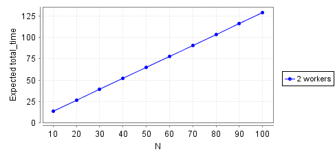
First throughput:
show data
| N | 2 workers | 1 worker |
|---|---|---|
| 10 | 14 | 20 |
| 20 | 27 | 40 |
| 30 | 39 | 60 |
| 40 | 52 | 80 |
| 50 | 65 | 100 |
| 60 | 78 | 120 |
| 70 | 91 | 140 |
| 80 | 103 | 160 |
| 90 | 116 | 180 |
| 100 | 129 | 200 |
You’d think it’d take half the total time to complete all tasks, but it’s actually closer to 2/3rds. We can only use both workers when the queue length is at least 2, so for most of each run we’re wasting a worker. If we saturated the queue by making the inbound rate much higher then the total time would converge to half the total time for one worker.
Now for latency:
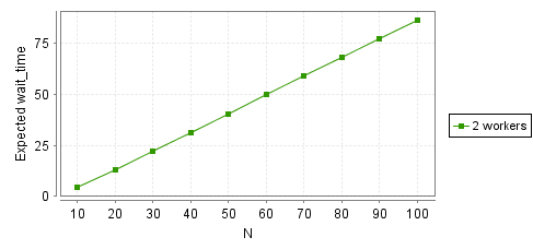
show data
| N | 2 workers | 1 worker |
|---|---|---|
| 10 | 5 | 29 |
| 20 | 13 | 97 |
| 30 | 22 | 190 |
| 40 | 31 | 305 |
| 50 | 41 | 436 |
| 60 | 50 | 584 |
| 70 | 59 | 746 |
| 80 | 68 | 922 |
| 90 | 77 | 1110 |
| 100 | 87 | 1310 |
For one worker the wait time was just about quadratic, while this is sublinear. The queue only jams if both workers stall out, which is a lot less likely. Going back to our 5 1 1 1 case, by the time the first worker has finished the first task the second worker has already processed the other three.
Generalizing the Model
Our model only covers a small part of the state space. We hardcoded the inbound probability, the outbound, and the number of workers. In particular I don’t like how we used the same probability for enqueuing and dequeuing. For all we know that leads to pathological results. A good spec should help us explore different parameters without us having to rewrite it.
The first change is the simplest: changing the inbound rate. PRISM lets us use expressions in guard clauses, so by adding a P_request constant we can vary in the inbound probability per step. All update probabilities must sum to 1, which is easy here.
const double P_request; // in [0, 1]

// ...

[enqueue] (queue < left & left <= N) ->
    P_request: (queue' = queue + 1)
    + (1 - P_request): true;
Changing the task processing rate is more complicated. Let’s say the probability of a worker processing a task is P. With two workers, there’s four possibilities:
- Both workers process a task:
p*p - W1 processes a task, W2 does not:
p*(1-p) - W2 processes a task, W1 does not:
(1-p)*p - Neither worker processes a task:
(1-p)*(1-p)
You can check that all the possibilities add up to 1. If we combine terms and simplify, we get
1 * p²(1-p)⁰: queue' = queue - 2
2 * p¹(1-p)¹: queue' = queue - 1
1 * p⁰(1-p)²: queue' = queue - 0
This might remind you of Algebra 1: (a + b)² = a² + 2ab + b². With a bit of combinatorics we can prove it’s the same. This is just the binomial expansion!4 The corresponding probabilities for 3 workers would be:
1 * p³(1-p)⁰
3 * p²(1-p)¹
3 * p¹(1-p)²
1 * p⁰(1-p)³
Not only can we use this to generalize the task processing rate, we can use this to scale up to an arbitrary number of workers. Unfortunately, that’s way too tedious to do by hand. So where’s what I did instead:
- [worker] // blah blah blah
+ $worker
And then I made a Python script write it for me. You can get the template and the script in this gist.
show generated spec
dtmc

const int N; // Max Tasks
const double P_request; // in [0, 1]
const double P_worker; // in [0, 1]
const int K; // [1, ]

module queues
  left : [0..N] init N;
  queue: [0..N] init 0;


[worker] (left >= 1 & ((queue >= 1 & K = 1) | (queue = 1 & K > 1))) ->
      1*pow(P_worker, 0)*pow(1-P_worker,1): (left' = left - 0) & (queue' = queue - 0)
    + 1*pow(P_worker, 1)*pow(1-P_worker,0): (left' = left - 1) & (queue' = queue - 1);

[worker] (left >= 2 & ((queue >= 2 & K = 2) | (queue = 2 & K > 2))) ->
      1*pow(P_worker, 0)*pow(1-P_worker,2): (left' = left - 0) & (queue' = queue - 0)
    + 2*pow(P_worker, 1)*pow(1-P_worker,1): (left' = left - 1) & (queue' = queue - 1)
    + 1*pow(P_worker, 2)*pow(1-P_worker,0): (left' = left - 2) & (queue' = queue - 2);

[worker] (left >= 3 & ((queue >= 3 & K = 3) | (queue = 3 & K > 3))) ->
      1*pow(P_worker, 0)*pow(1-P_worker,3): (left' = left - 0) & (queue' = queue - 0)
    + 3*pow(P_worker, 1)*pow(1-P_worker,2): (left' = left - 1) & (queue' = queue - 1)
    + 3*pow(P_worker, 2)*pow(1-P_worker,1): (left' = left - 2) & (queue' = queue - 2)
    + 1*pow(P_worker, 3)*pow(1-P_worker,0): (left' = left - 3) & (queue' = queue - 3);

[worker] (left >= 4 & ((queue >= 4 & K = 4) | (queue = 4 & K > 4))) ->
      1*pow(P_worker, 0)*pow(1-P_worker,4): (left' = left - 0) & (queue' = queue - 0)
    + 4*pow(P_worker, 1)*pow(1-P_worker,3): (left' = left - 1) & (queue' = queue - 1)
    + 6*pow(P_worker, 2)*pow(1-P_worker,2): (left' = left - 2) & (queue' = queue - 2)
    + 4*pow(P_worker, 3)*pow(1-P_worker,1): (left' = left - 3) & (queue' = queue - 3)
    + 1*pow(P_worker, 4)*pow(1-P_worker,0): (left' = left - 4) & (queue' = queue - 4);


  [] (left = 0) -> true;

  [enqueue] (queue < left & left <= N) ->
    P_request: (queue' = queue + 1)
    + (1 - P_request): true;
endmodule

rewards "wait_time"
  [worker] queue > K: queue - K;
endrewards

rewards "total_time"
  [worker] left > 0: 1;
endrewards
I snuck in one more change there: I modified the guard clause to use a new constant K. I didn’t like how I hardcoded the number of workers we were using, so now K is the number of workers we have. That way if you want to play with it yourself you don’t have to modify the spec to switch between 1 or 2 (or 3 or 4) workers.
Conclusion
This was a simple model of task queues. We didn’t cover priority, error handling, multiple queues, etc. Nonetheless, the spec was good enough to show how nonlinear latency is and how adding more workers can have a dramatic effect.
If you’re interested in PRISM, you can download it here. I’m happy to answer simple questions or provide tips if needed. If you’re interested in the broader mathematical theory of task queues, you’ll want to look into queueing theory.
I shared the first draft of this essay on my newsletter. If you like my writing, why not subscribe?
- Here we are using it as cost, not reward. But since these are operationally the same thing PRISM only has syntax for reward functions. [return]
- “Wait, how can it be the same inbound/outbound rate if the step is an abstract model of time?” Good question. In this case I set up the model in a precise way to make sure this works. In practice you’d write your PRISM spec in a “generic” way that’s a little tougher to read but easier to design correctly. I used the “more elegant” spec to keep the focus on task queues. [return]
- The numbers are slightly different if we make the reward
(queue)instead of(queue-1), but the trend is the same. [return] - Given N workers, there are
N choose Kdifferent ways for exactly K workers to process a task in a given tick, and each case has a probability ofp^K*(1-p)^(N-K). [return]